Explore the Scientific R&D Platform

Try Now
Pricing
MENU
Try Now
Pricing

How to calculate sample size in 5 steps:
& how to use a sample size calculator

Ensure your sample size determination is of significance by following these 5 steps

Why is sample size calculation important?

Firstly, a study which is too small is more likely to generate inconclusive, incorrect or spurious results. This is because a smaller sample size will generate estimates which have higher variation. These estimates will then be less useful in modelling and understanding the real underlying questions of interest in a study.

Secondly, studies which are more likely to fail due to inadequate sample size are considered unethical. This is because exposing human subjects or lab animals to the possible risks associated with research is only justifiable if there is a realistic chance that the study will yield useful information. Additionally, a study which is too large faces the same ethical problem and will also waste scarce resources such as money, subjects and time.

For these reasons, a sample size justification is a standard part of study design. Whether it is the Nature Publishing Group or the Federal Drug Administration (FDA), a study which does not justify its sample size has a higher chance of rejection, scrutiny or failure.

  • Statistical power is the most commonly used metric for sample size determination.
  • The power is the probability that the study will be able to detect a true effect of a drug or intervention of a specified size or greater.
  • In statistical hypothesis terms, power is the probability of rejecting the null hypothesis when it is false.

The 5 steps to calculate sample size for a clinical trial

In this article we will outline the 5 step process for determining the appropriate sample size or power for your study. At Statsols, these are called the “5 Essential Steps for Sample Size” and the outline of these steps is as follows:

NOTE: You can click on each heading to be brought to that section.
Step 1 PLAN YOUR STUDY - Sample Size Calculator
Clean & Elegant
Fully Responsive

Step 1. Plan Study

  • What question(s) are you trying to answer?
  • What is the primary outcome(s)?
  • What statistical method(s) will you use?
Step 2  Specify Parameters - Sample Size Calculator
Clean & Elegant
Fully Responsive

Step 2. Specify Parameters

  • What parameters are needed for your statistical method? E.g. significance level, standard deviation, intracluster correlation.
  • How to deal with parameters which are known or unknown before the study?
  • What is your best estimate for these parameters?
Step 3 Choose Effect Size- Sample Size Calculator
Clean & Elegant
Fully Responsive

Step 3. Choose Effect Size

  • What effect size is appropriate for your study?
  • What criteria can be used to select the appropriate effect size?
  • What is the expected effect size for the proposed treatment or intervention?
Step 4 Compute Sample Size  - Sample Size Calculator
Clean & Elegant
Fully Responsive

Step 4. Compute Sample Size or Power

  • When to calculate sample size and when to calculate power?
  • What power is appropriate for a study?
  • What adjustments may need to be made to the sample size?
Step 5 Explore Parameter Uncertainty   - Sample Size Calculator
Clean & Elegant
Fully Responsive

Step 5. Explore Uncertainty

  • Why exploration is an important step for regulatory approval
  • How to explore uncertainty in parameter estimates (e.g. effect size, SD) and effect on sample size?
  • Innovative approaches to exploring uncertainty in sample size determination

How to calculate sample size for clinical trials (detailed guide)

Step 1. Plan Your Study

Planning the study involves establishing the purposes of the study, what is going to be measured to fulfil those purposes and what statistical methods and assumptions that go into extracting those from your study design. Below are some common questions and answers that arise at this stage.

What Do You Want To Answer?

It must be established what the study question, or questions are. The study questions inform what conclusions can be made at the end of the study. It is vital at an early stage we establish “what do we want this study to tell us?”. For example, in an oncology trial, we may want to see if the new treatment reduces mortality, or in a classroom intervention we may be interested in seeing if the intervention improves grades.

Establishing the study question is vital as it has knock-on effects on all the other assumptions and choices discussed below that will be made when planning the study.

What is the primary outcome of the study?

The next thing you’ll ask, having established your main study question(s), is what is the primary outcome (or primary outcomes) in the study. This is the endpoint we will measure in order to make a conclusion about the study question. In an oncology trial, that might be the mortality rate in the treatment group and the control group; or in an educational study it might be the measurement of grades or the attendance.

Often this is simple to define but in some cases it can be more complex. For example, where there are multiple endpoints to measure, or where we want to make a composite measure of the outcome to make conclusions about the study question. Guidance on the issue of estimands can illustrate how this issue can be more complex than expected.

The primary outcome chosen will also decide the type of data that will be analysed at the end of the study. When a mortality rate is the endpoint, data is often of a binary nature, and thus the data take the form of proportions. However, another researcher may choose to analyse the time to the mortality event. In a trial where the value of a biological response, such as change in lung function, is the primary endpoint, the data would often be continuous in nature, and thus comparison could be made via the means of the different arms or groups in the trial.

What kind of grouping structure will the study have?

Once this is completed, there are many other design decisions to make. Will the study be observational in nature, versus a controlled trial; how many groups will be compared in this particular study; will subjects in different arms of the study be paired or analysed separately; will subjects be randomized individually to treatments, or will hospitals or other clusters be randomized to the treatments, with all subjects in each cluster receiving the same treatment. Each of these choices will influence the statistical choices available and thus the relevant sample size calculation.

What type of statistical method and hypothesis will be used?

Once all these assumptions are made, a statistical hypothesis test needs to be chosen. This is a statistical model that will be used to make conclusions about the study question based on the primary outcome. For comparing two means, a Z-test or t-test might be used, whereas for comparing two proportions, a Chi-square test may be most appropriate.

Regardless of the method chosen, it is important to make the choice of which statistical test to use before the beginning of the study. If this choice is not made prior to the study, it can be difficult to accurately assess the sample size required for the study and will make study approval more difficult.

The focus on this guide is on statistical power which is tied to hypothesis testing but sample size can also be based on other considerations such as confidence interval width or cost-theoretic approaches. More details on these approaches are available elsewhere on the nQuery website.

Once these decisions have been made and the study protocol has been fully specified, you can move on to step two. 


Step 2. Specify Parameters 

Step two involves specifying the analysis parameters for the study.

 The analysis parameters are assumptions that need to be made about the statistical method to make a sample size justification for the study. Each study design has different analysis parameters that must be estimated in the design stage of the study.

What are the two primary types of parameters used in sample size determination?

Pre-specified parameters and unknown parameters are the primary types of parameters used in sample size determination

Pre-specified parameters are those which can be known with certainty before the study as they are part of the study planning process. 

For example, an analysis parameter that is seen in almost every sample size justification is the significance level, alpha. There are often several other similar parameters which are required for each particular model such as the number of categories in a study using analysis of variance (ANOVA). Standard values can often be used for these, such as 0.05 for the significance level.

Unknown parameters are those which have uncertainty about what value they will have in the final analysis. In the majority of cases, there is no such standard value and a value which estimates the parameter for the current study population as best as possible is needed.

For example, in the comparison of means an assumed value will often be needed for the standard deviation. In a cluster randomized trial, a parameter called the intracluster correlation will need to be specified. In comparing two incidence rates, a dispersion parameter is often used.

These values are unfortunately often quite difficult to choose, as the study has not yet taken place, and thus the exact value of the standard deviation in the treatment group, for example, is not yet known. Pilot studies, previous studies, pre-existing data and the academic literature are often recommended to ascertain the most commonly used and most plausible parameter values from studies and data of the most relevance. There will usually be uncertainty over the chosen value of these specified parameter values and dealing with this uncertainty will be explored in Step 5 below

Step 3. Choose Effect Size

Once the analysis parameters are specified, you can move on to step 3, which is to specify the effect size for the sample size calculation. This is the difference in the primary outcome value used in the sample size calculation that the clinical trial or study is designed to reliably detect.  

A standardized effect size measures the magnitude of a treatment effect without units, allowing a more direct and comparable measure of the expected degree of the effect across different studies. For the two-group t-test, the standardized effect size is the difference between the two means divided by the common within-group standard deviation, so an effect size of 1.0 would indicate a difference between the two means equal to one standard deviation. A very common standardized effect size metric is Cohen’s effect size, where “small”, “medium” and “large” effects are defined as standardized effect sizes of 0.2, 0.5 and 0.8 respectively.

An unstandardized effect size is simply the raw effect – such as a difference or ratio between two means, two rates or two proportions. In general, the greater the true effect, the easier it will be to detect the difference using the sample selected for the clinical trial. The unstandardized effect size gives a more direct study-specific measure of the effect size we expect in the study. It allows a greater degree of flexibility when assessing and exploring the appropriate sample size for the study in combination with unknown parameters in Step 2.

Why is the effect size important in a clinical study?

Selecting an appropriate effect size is one of the most important aspects of planning a clinical trial. If the difference used in the calculation is smaller than the true difference, a larger sample size than necessary will be required to detect the difference. This is a big issue, as from an ethical point of view, no more participants than necessary should be recruited to answer the research question. Recruitment for clinical trials can often be time-consuming and resource intensive, with every extra patient increasing the cost of the trial.

If the effect size used in the calculation is larger than the true effect, then the sample size calculated at the beginning of the trial will not be enough to achieve the target power. Unless it is planned at the beginning of the trial, the sample size cannot be increased, and thus there is a large risk the trial will fail.

The effect size also directly lays out the real quantitative objective of the study and allows an opportunity to consider what success would mean in the context of your study.

How to select the appropriate effect size?

Various approaches and interpretations exist for how to find the effect size value. In addition, there are many different opinions regarding what the effect size should be. For other parameters, such as the standard deviation, the aim is to obtain the most accurate estimate possible, whereas for the effect size, this is not as clear.

What are the two main approaches for specifying the effect size?

1: Select a clinically relevant difference (i.e. a difference that would be important from a clinician’s or patient’s perspective)
2: Select a realistic difference based on prior evidence and information

It can be argued that the selected effect size should fulfil both of these points, such that the difference is clinically relevant and biologically plausible. The recommendation from many experts in the field is to power the study or clinical trial for the minimum difference worth detecting. This could be interpreted as lower bound for the effect size which would still be considered clinically relevant and should ideally be defined in conjunction with the pre-existing evidence and expert option.

Once the reasoning behind the effect size has been chosen, you still must decide what this value itself should be. Many formal methods are available to determine the effect size for a clinical trial. 

  • Pilot study
  • Health economic method - consider net benefit of treatment including cost
  • Eliciting expert opinion - such as from clinicians
  • Systematic review and meta - analysis of evidence
  • Standardized effect size - such as Cohen’s d
  • Distribution method - choose value larger than imprecision of measurement

In general, the distribution method is not as good as other methods, and so other methods should be given preference. In addition, the pilot study method should only be used in conjunction with another method, as the error in measurement will be too large for the value to be depended upon alone. The final choice of which methods to use will most often just depend on the availability of the information and resource considerations.

In recent years, new methods have appeared to deal with the influence of uncertainty around the effect size of a new treatment. These include methods such as Bayesian Assurance, where the effect size is parameterized in the form of a distribution of values as opposed to a single value, and unblinded sample size re-estimation, where the effect size can be updated midway through a study based on data collected up to that point, are focused on minimising and accounting for the uncertainty around the effect size.

These methods will be covered in more detail in Step 5.

Step 4. Compute Sample Size

Once step 3 is completed, and the effect size is specified, you can move onto step 4, which is to compute the sample size or power for the study.

The most common situation is that you want to find the required sample size for a given power. In general, increasing sample size is associated with an increase in power.

Traditionally, in clinical trials, 80% power would have been chosen. This would give a 1 in 5 chance of not rejecting the null hypothesis when indeed it is true. Choosing a power of 80% runs a reasonable risk of an underpowered study, however, if the true effect is smaller than initially thought, or other parameters are inaccurately estimated.

More recently statisticians such as Steven Julious have recommended aiming for 90% power, which slightly mitigates the risk of an underpowered study, as even if there are dropouts, or the standard deviation or other parameters are more extreme than anticipated, there will still be greater than 80% power. In addition, two confirmatory trials are usually required for regulatory approval and two trials with 90% power will have at least 80% power to find a significant effect in both studies based on the two trials’ outcomes being independent and thus the combined power being equal to 0.9 squared i.e. 81%.

You may also want to consider some additional adjustments to the sample size to deal with known complications that may occur in a study. The most common adjustment is for dropout with the most common adjustment being dividing the original sample size estimation by one minus proportion expected to dropout during the course of the study. This is illustrated in the example below.

Certain sample size determination methods allow for more complex dropout patterns such as those used in time to event analyses and these cases dropout will be treated as if it were an unknown parameter from Step 2. Other adjustments can similarly be made for issues such as the treatment crossover or the effect of delayed accrual.

Sometimes, however, the sample size may be constrained by study costs such as the drug manufacture cost or the size of the available population. This may be particularly relevant in academic settings with smaller budgets. In this case, it can be useful to know what the power would be, given the assumptions from steps 2 and 3, and the available sample size. This will establish how viable the study is, and how likely it is to give useful conclusions for the current study.

What is an example of a sample size calculation?

An example from Sakpal (2010) will now be examined. “An active-controlled randomized trial proposes to assess the effectiveness of Drug A in reducing pain. A previous study showed that Drug A can reduce pain score by 5 points from baseline to week 24 with a standard deviation (σ) of 1.195. A clinically important difference of 0.5 as compared to active drug is considered to be acceptable.”

For this test we would like to find the sample size required for 80% power, with a two-sided 5% level of significance.

The formula required is:

Formula Required for Sample Size

Where n  = required sample size in each group, μ1is the mean change in pain score from baseline to week 24 in Drug A = 5, μ2is the mean change in pain score from baseline to week 24 in Drug B = 4.5, the clinically important difference μ1-μ2= 0.5, σ is the standard deviation = 1.195.

Zα2is the standard normal z-value for a significance level α = 0.05, which is 1.196. Zβis the standard normal z-value for the power of 80%, which is 0.84.

Using the formula above, the required sample size per group is 90, and thus the total sample size required is 180.

This calculation can also be completed using the nQuery software, by selecting the “Two Sample Z-test” table, and entering the parameters above. The calculation again shows that a sample size of 90 is required in each group.

How to calculate two means - nQuery sample size software screenshot 2


In addition, we will add an assumed total dropout of 10% during the course of the study. To calculate the adjusted sample size, we divide the total expected sample size by one minus the proportion expected to dropout (0.10 in this case). We thus divide 180 by 0.9 to give a sample size adjusted for dropout of 200 in this study.

Step 5. Explore Parameter Uncertainty  

Once steps 1 to 4 have been completed, and the appropriate sample size or relevant power has been found, you can move onto step 5 which is to explore the uncertainty in your sample size design.

The unknown parameters and effect size that have been defined in steps 2 and 3 are just that - estimates. It is not known what the true value of these parameters should be. If all these parameters were known, there would be no need to run the clinical trial! If the parameters are inaccurate, we risk the possibility of underpowering the study and not having a large enough sample size to find the effect size or we may overpower and subject too many people to what may be an ineffective treatment. 
 
Traditionally, this uncertainty would have been explored primarily using sensitivity analysis.  A sensitivity analysis is a part of planning a clinical trial that is easily forgotten but is extremely important for regulatory purposes and publication in peer-reviewed journals. It involves analyzing what effect changing the assumptions from parts 2, 3 and 4 would have on the sample size or power in the particular sample size or power calculation. This is important as it helps in understanding the robustness of the sample size estimate and dispels the common overconfidence in that initial estimate.

Some parameters have a large degree of uncertainty about them. For example, the intra-cluster correlation is often very uncertain when based on the literature or a pilot study, and so it’s useful to look at a large range of values for that parameter to see what effect that has on the resulting sample size. Moreover, some analysis parameters will have a disproportionate effect on the final sample size, and therefore seeing what effect even minor changes in those parameters would have on the final sample size is very important.

When conducting a sensitivity analysis, a choice has to be made over how many scenarios will be explored and what range of values should be used. The number of scenarios is usually based on the amount of uncertainty and sensitivity to changes and when these are larger, more scenarios should be explored. The range of values is usually based on a combination of the evidence, the clinical relevance of different values and the distributional characteristics of the parameter. For example, it would be common to base the overall range on the range of values seen for a parameter seen across a wide range of studies or to base it on the hypothetical 95% confidence interval for the parameter based on previous data or a pilot study. For effect size, clinically relevant values will tend to be an important consideration for which range of values to consider.

However, it is important to note that there is no set rules for which scenarios should be considered for a sensitivity analysis and thus sufficient consideration and consultation should be used to define the breadth and depth of sensitivity suitable for the sample size determination in your study.

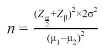
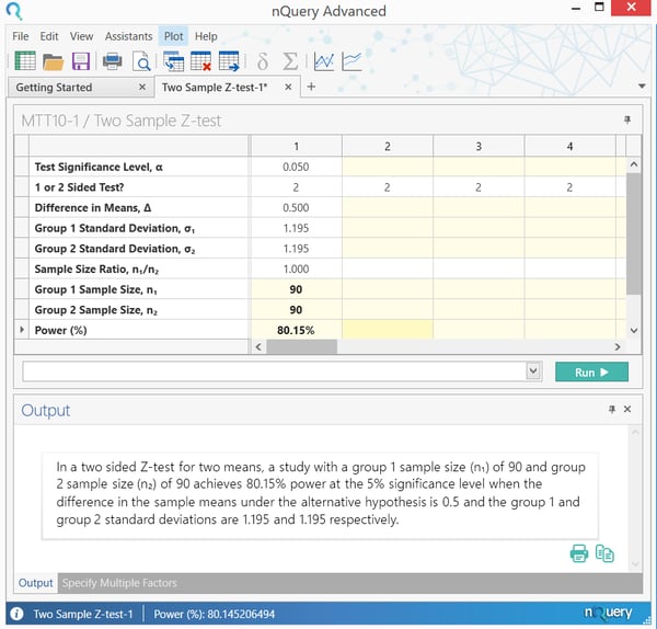
A sensitivity analysis for the example above is shown below. Here, the standard deviation in the group receiving the new treatment is varied, to assess the effect on the sample size required in that group. The sample size in the control group remains at 90, and we are always aiming for 90% power. The plot shows that as the standard deviation increases, the sample size required increases dramatically. If the standard deviation is underestimated, a larger sample size is required to reach 80% power, and thus the trial will be under powered.

For σ= 1.5,  1 = 142, while for σ= 2.0,  1 = 253. This shows the importance of estimating the standard deviation as accurately as possible in the planning stages, as it has such a large impact on sample size and thus power.two means plot - nQuery Sample Size Software

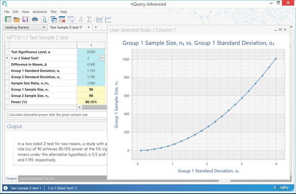
Though sensitivity analysis provides a nice overview of the effect of varying the effect size or other analysis parameters, it does not present the full picture. It usually only involves assessing a small number of potential alternative scenarios, with no set official rules for choosing scenarios and how to pick between them.

How can we improve upon or supplement the process of sample size determination?

A method often suggested to combat this problem is Bayesian Assurance. Although this method is Bayesian by nature, it is used as a complement to frequentist sample size determination.

What is Bayesian Assurance?

Assurance, which is sometimes called “Bayesian power” is the unconditional probability of significance, given a prior or prior over some particular set of parameters in the calculation. These parameters are the same parameters detailed in steps 2 and 3 above. 

In practical terms, assurance is the expectation of the power over all potential values for the prior distribution for the effect size (or other parameter). Rather than expressing the effect size as a single value, it is expressed as a mean (the value the effect size is most likely to be - usually the value used in the traditional power calculation) and a standard deviation (expressing your uncertainty about that value). If the power is then averaged out over this whole prior, the result is the assurance. This is often framed as the “true probability of success”, “Bayesian Power” or “unconditional power” of a trial.

How does Bayesian Assurance let us explore uncertainty?

In a sensitivity analysis, a number of scenarios are chosen by the researcher, and assessed individually for power of sample size. This gives a clear indication of the merits of the individual highlighted cases, but no information on other scenarios. With assurance, the average power over all plausible values is determined by assigning a prior to one or more parameters. This provides a summary statistic for the effect of parameter uncertainty, but less information on specific scenarios.

Overall, assurance allows researchers to take a formal approach to accounting for parameter uncertainty in sample size determination and thus create an opportunity to open a dialog on this issue during the sample size determination process. The definition of the prior distribution also allows an opportunity to formally engage with previous studies and expert opinion via approaches meta-analysis or expert elicitation frameworks such as the Sheffield Elicitation Framework (SHELF).

What is an example of an Assurance/Bayesian Power calculation for assessing the effect of a new drug?

O’Hagan et al. (2005) give an example of an assurance calculation for assessing the effect of a new drug in reducing C-reactive protein (CRP) in patients with rheumatoid arthritis.

The outcome variable is a patient’s reduction in CRP after four weeks relative to baseline,
and the principal analysis will be a one-sided test of superiority at the 2.5%
significance level. The (two) population variance … is assumed to be … equal to
0.0625. … the test is required to have 80% power to detect a treatment effect of 0.2,
leading to a proposed trial size of n1 = n2 = 25 patients
 …"

For the calculation of assurance, we suppose that the elicitation of prior information … gives the mean of 0.2 and variance of 0.0625. If we assume a normal prior distribution, we can compute assurances with m = 0:2, v = 0.06 … With n = 25, we find assurance = 0.595.

The calculation of sample size, and subsequently assurance, can be demonstrated easily in nQuery. The sample size calculation again used the “Two Sample Z-test” table.

o'Hagan means screenshot - nQuery sample size software

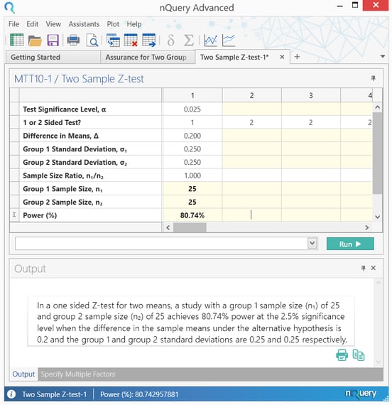
This calculation shows that a sample size of 25 per group is needed to achieve power of 80%, for the given situation.

The assurance calculation can then be demonstrated using the “Bayesian Assurance for Two Group Test of Normal Means” table. To view the list of Bayesian Sample Size Procedures in nQuery, click here.


Start your 14 day free trial of nQuery

nQuery is the standard for fixed-term, Bayesian & Adaptive trials

 
50k Users
Commercial, academic &
government organizations
Successful Trials
Recognized by the FDA, EMA

& other regulatory bodies

Recommended articles for you